5 Deep Learning and Neural Architectures
5.1 Overview and Historical Notes
Initial AI systems are based on the definition of formal systems (logic, knowledge base, etc.).
Several artificial intelligence projects have sought to hard-code knowledge about the world in formal language.
Difficult to list rules for very large number of situations.
Some rules might also not be possible to be codified given the sheer complexity of the world.
\(\blacktriangleright\) However note: recent developments in combining deep learning and symbolic AI (very open field of research at the moment!).
5.2 Abstract/Formal Tasks vs Intuition
Abstract and formal tasks that are among the most difficult undertakings for a human being are among the easiest for a computer.
Computers have long been able to defeat even the best chees player but only recently have begun matching some of the abilities of average human beings to recognise objects or speech.
Much of human knowledge is about unstructured “inputs” (e.g. sensory data).
Computers need to capture this same knowledge in order to behave in an intelligent way.
5.3 Extracting Patterns from Raw Data
AI systems need the ability of acquiring their own knowledge by extracting patterns from raw data.
Usually, this capability is referred to as machine learning.
Machine learning allows computer systems to learn through data and experience.
Examples: naive Bayes, logistic regression, decision tree, random forest, etc.
5.4 Representation and Features
The performance of these algorithms depends heavily on the representation of the data they are given.
For example, in order to determine if a patient has a certain disease or not we can input certain physiological indicators (with thresholds, for example, temperature higher than 37.5C) and/or the presence of absence of certain symptoms.
Each piece of information included in the representation of the patient is called known as a feature.
A machine learning algorithm (let’s say logistic regression) learns how each of these features of the patient are linked to a certain condition.

In this case features might be occurrences or not of certain words, formatting, length of the message or other information related to the email protocols.
We can build a vector of values (continuous and discrete) representing each email. Each element of the vector will be associated to one feature.
Many artifiicial intelligence tasks can be solved by designing the right set of features.
However, for many tasks it is difficult to know what features should be extracted.
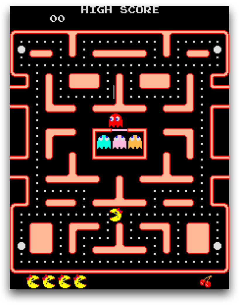
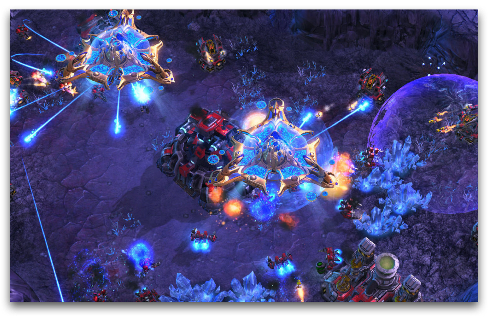
- Think about identificaiton of a photo, emotion in a voice of a speaker, understanding images of a road, playing a complex videogame (e.g. Starcraft).
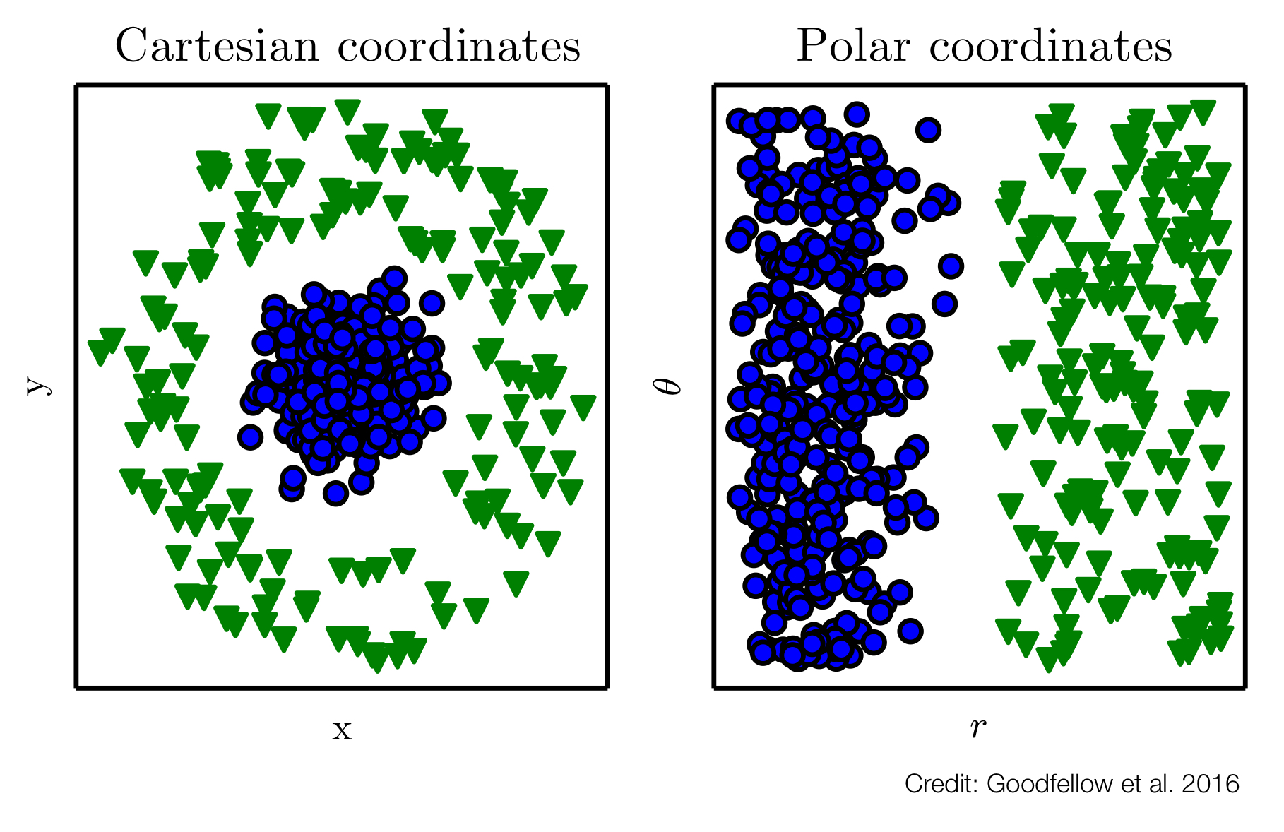
Note: it is not only about the features themselve, but how the information is structured and “represented”: Machine learning on Roman numbers is probably not a good idea.
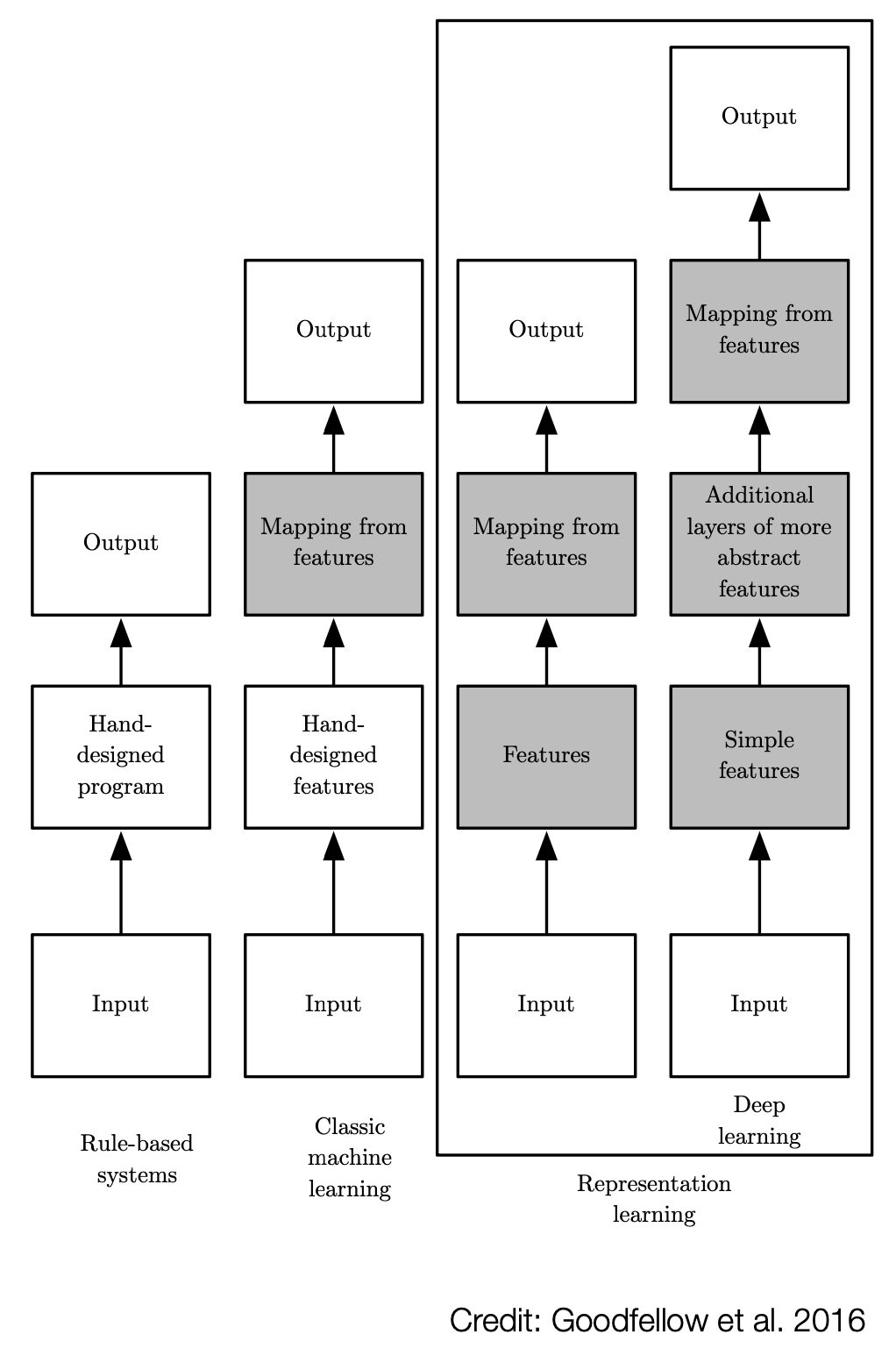
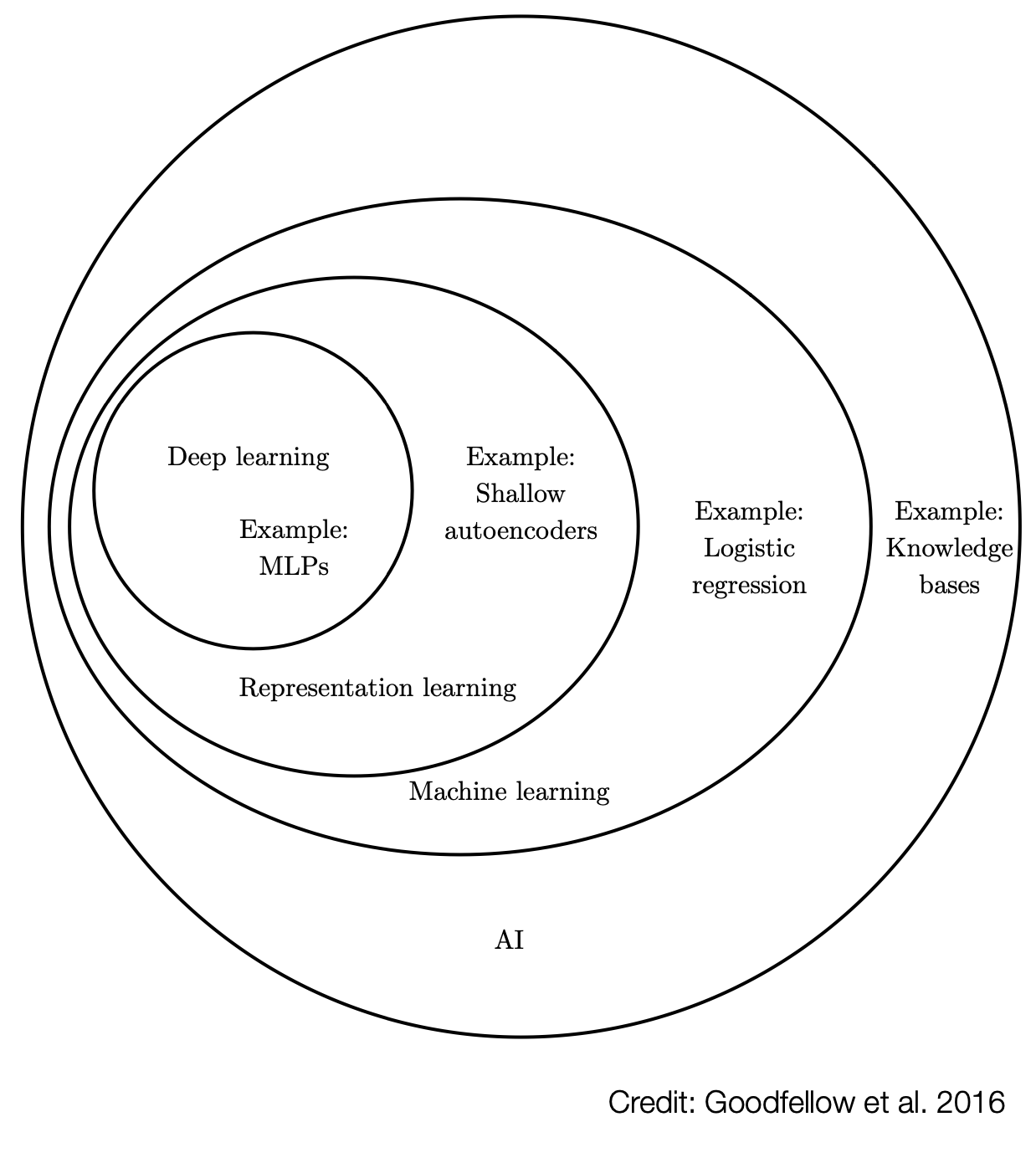
5.5 Representation Learning
One solution to this problem is to use machine larning to discover not only the mapping form representation to output but also the representation itself.
This approach is usually known as representation learning.
Learned representation often results in much better performance than can be obtained with hand-made representations.
5.6 Factors of Variation
When designing features or algorithms for learning features, out goal is to separate the factors of variation that explain the observed data.
In this context, we use word factors to refer to separate sources of information that are useful for the machine learning task at hand.
Such factors are often quantities that are not directly observed.
They are often unobserved (or latent) and they affect the observable ones.
Some of them might be linked to human constructs (e.g. the colour of an object) and other might not. In the latter case, the factors might not be easily interpreted by a human (see also the problem of AI interpretability).
Some factors of variantion affect all the piece of information we have (for example angle of view of a car).
We need to disentagle the factors that allow us to successfully perform the machine learning task and extract representations that are not affected by factors of variation that are not “useful” for the task.
For example, if we need to classify a car vs truck, the angle itself is not fundamental for the classification.
We need a tool that learns to “ignore” that factor of variation.
5.7 Deep Learning
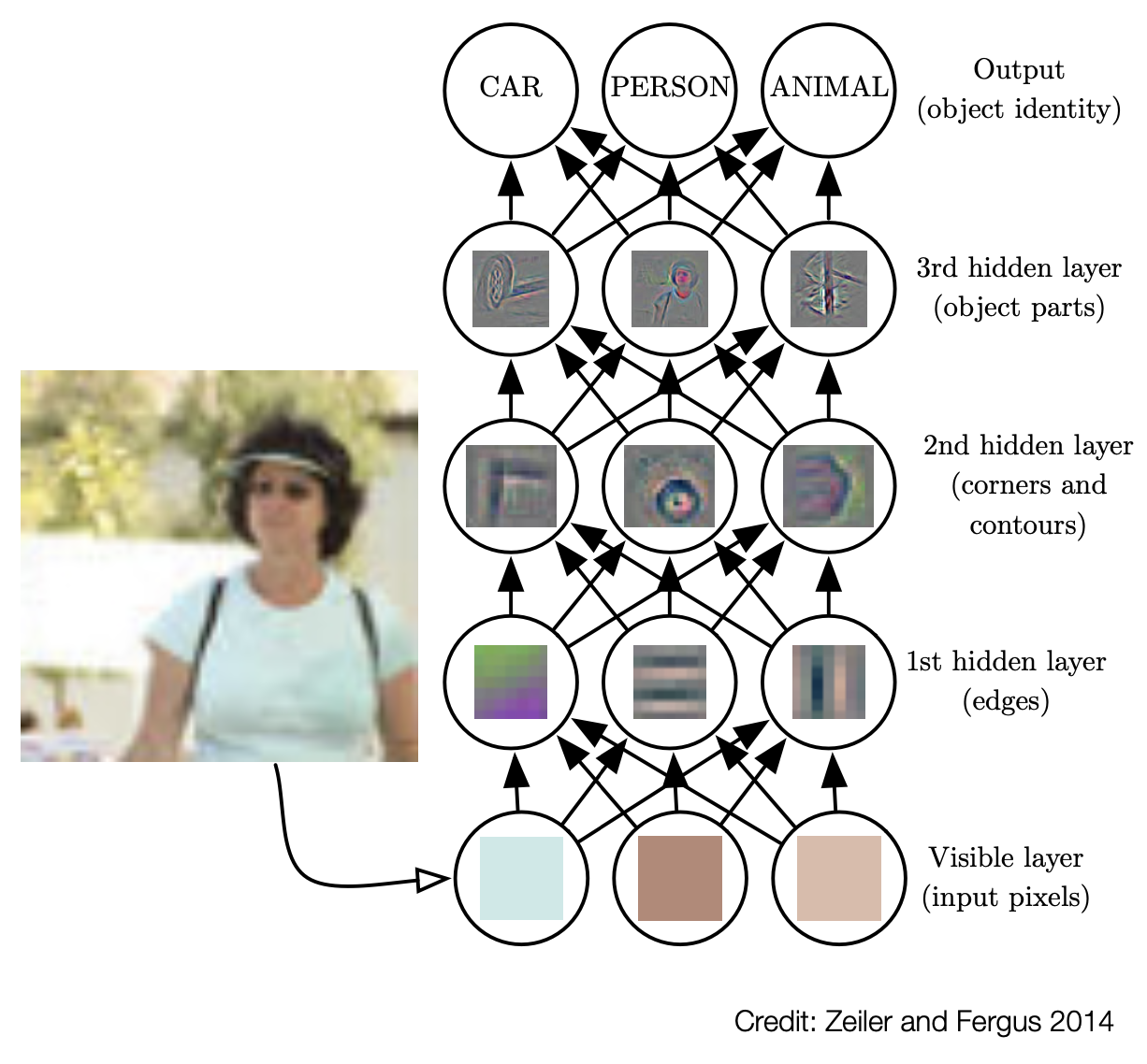
Deep Learnin address this problem of representation learning by introducting representations that are expressed in terms of other, simpler representations.
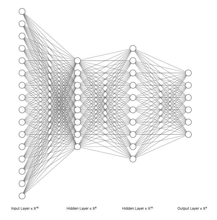
Classic example of deep learning model is the feedforward deep network (or multi-layer perceptron).
Plase note: a multilayer perceptron at the end is a (complex) mathematical function mapping input values to output values.
This function is the result of combining several simpler functions in the intermediate nodes.
Until now, we have considered one of the possible interpretation of deep learning, i.e. that it allows to learn the right representation for the data.
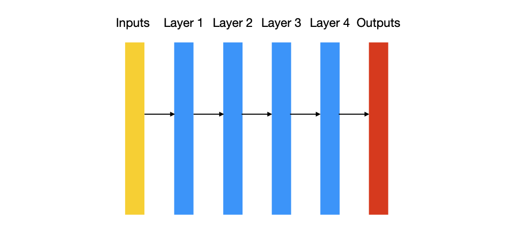
Another possible perspective on deep learning is that depth enables a computer to learn a multi-step computer program.
- Each layer of the network can be thought as the state of the computer’s memory after executing a set of instructions in parallel.
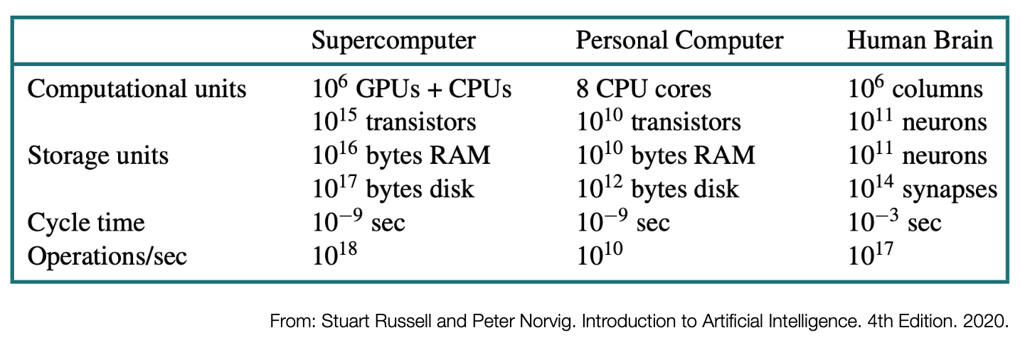
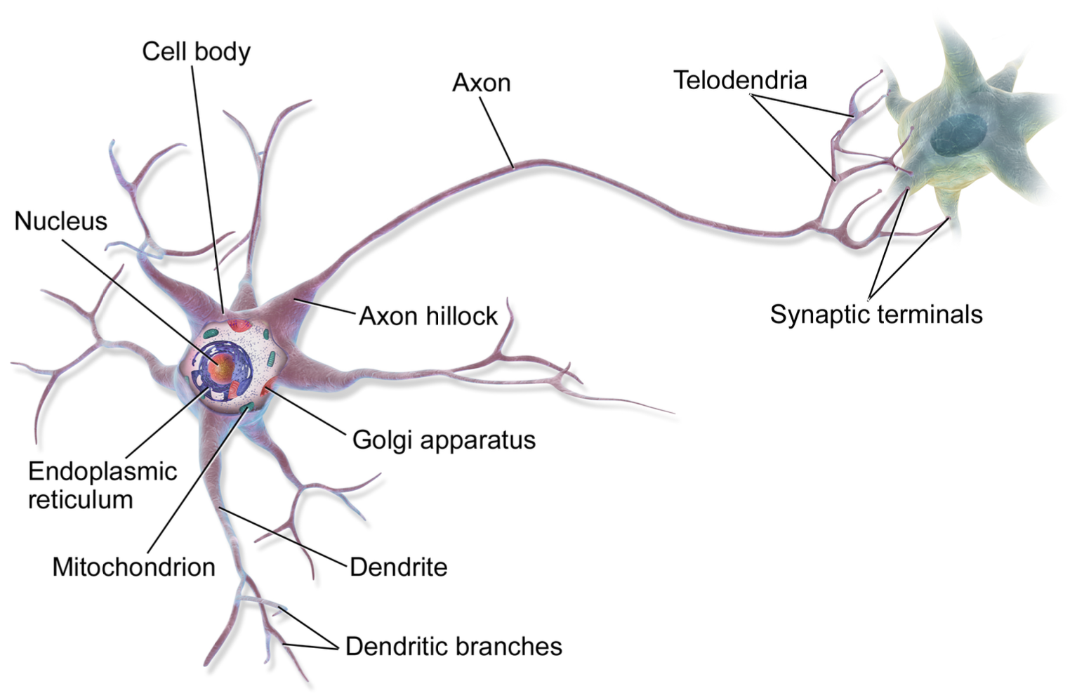
5.8 Computers and Brains
5.9 From Theories of Biological Learning to Deep Learning
There are three waves:
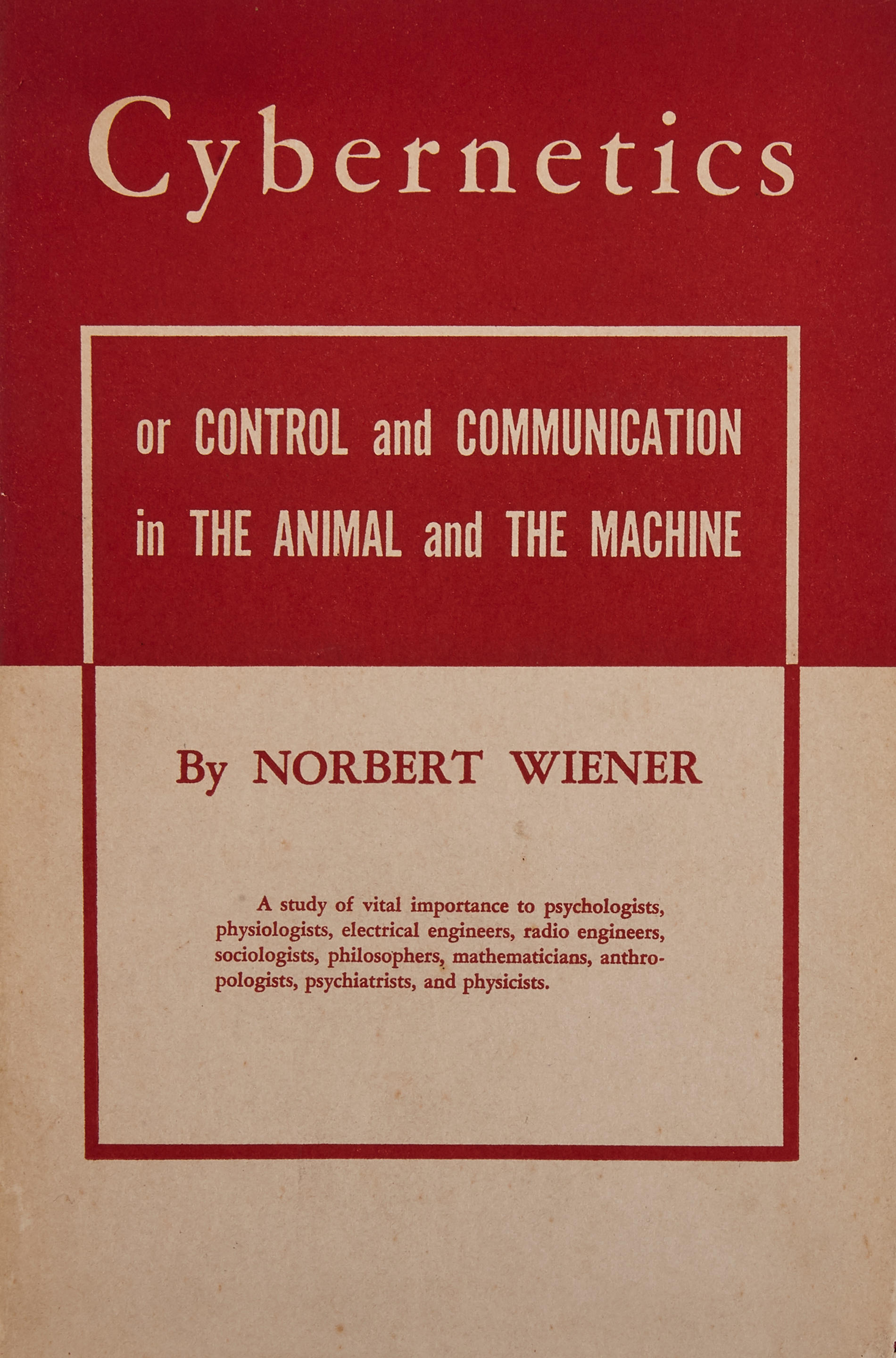
Cybernetics (1940s – 1960s)
Connectionism (1980s – 1990s)
Deep Learning (2006 – today)
Some of the earliest learning algorihtms were intended to be computational models of the brain. As a result, one of the names used for deep learning is artificial neural networks (ANNs).
5.10 Artificial Neural Networks and Neuroscience
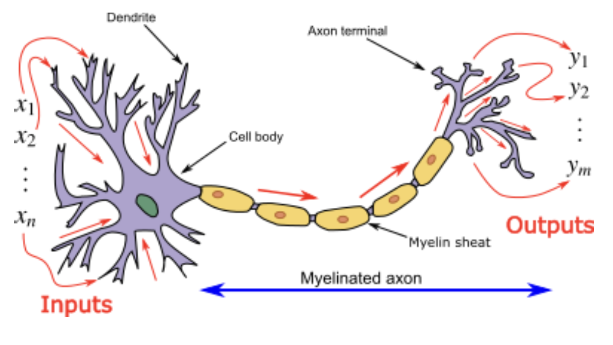
The earliest predecessors of modern deep learning were simple linear models motivated from a neuroscience perspective.
These models were designed to take a series of \(n\) input values \(x_1, x_2, \dots, x_n\) and associate them to an output \(y\).
These models would be based or learn a set of weights:
\(y = f(\mathrm{x}, \mathrm{w}) = w_1 x_1 + \dots + w_n x_n\)
5.11 The McCulloch-Pitts Neural Model
In “A Logical Calculus of the Ideas Imminent in Nervous Activity” (1943), McCulloch1 and Pitts2 suggested a mathematical cognitive model.
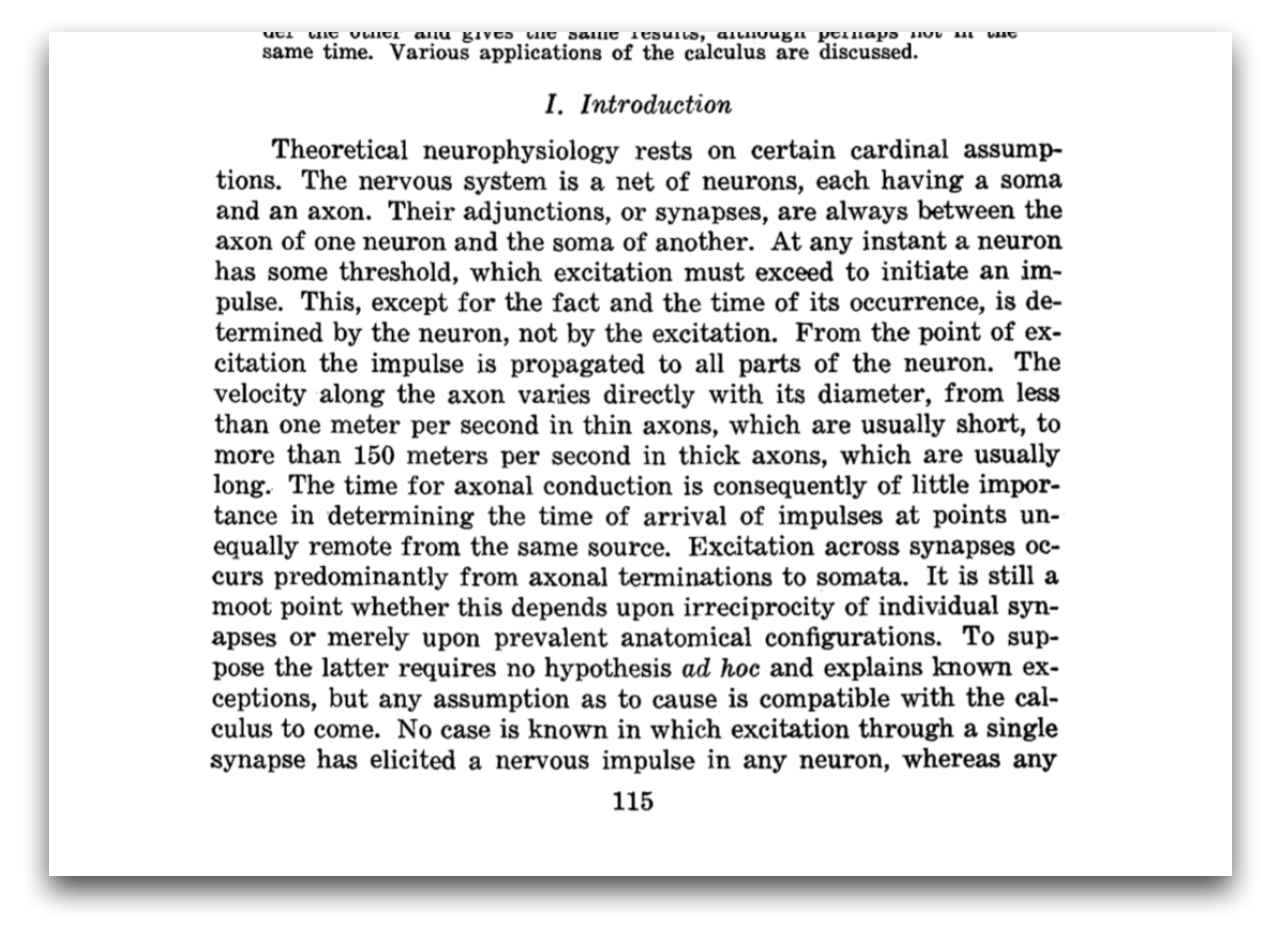
This can be considered the original inspiration of current deep learning models.
The set of operations is defined over two values:
- True (1)
- False (0)
The calculus contained NOT, AND, OR. By changing the (fixed) values of the weights, you can obtain different functions.
MCulloch-Pitts’ Model of Neuron
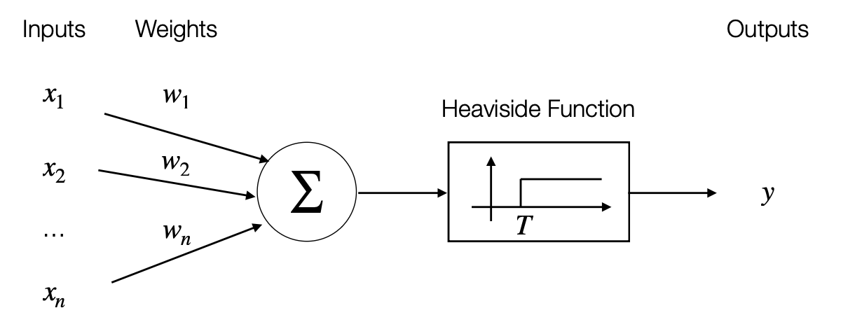
McCulloch-Pitts Model of Neuron:
the values of the weights are fixed.
5.12 The Hebb’s Neural Model
Hebb’s Law
From Hebb3 ’s “The Organization of Behavior” (1949): “When an axon cell A is near enough to excite cell B and repeatedly or persistently takes part in firing it, some growth process or metabolic change takes place in ore or both cells such as that A’s efficiency, as one of the cells firing B is increased”.
This is usually referred as Hebb’s Law.
First simulations of artificial neural nerworks in 1950s based on Hebb’s model.
Weights of the models are also called synaptic connectivity.
Hebb’s Model of Neuron
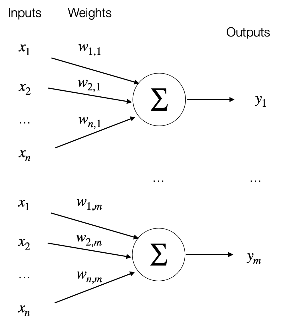
The Hebbian network model has \(\mathbf{n}\)-node input layer: \[\mathrm{x} = [x_1,x_2,\dots,x_n]^T\] and an \(\mathbf{m}\)-node output layer: \[\mathrm{y} = [y_1,y_2,\dots,y_m]^T\]
Each output is connected to all input as follow: \[y_i = \sum^n_{j=1} w_{j,i}x_j\]
The learning rule is the following: \[w_{j,i}^{new} \leftarrow w_{j,i}^{old} + \mu x_j y_i\] \(\mu\) is the learning rate.
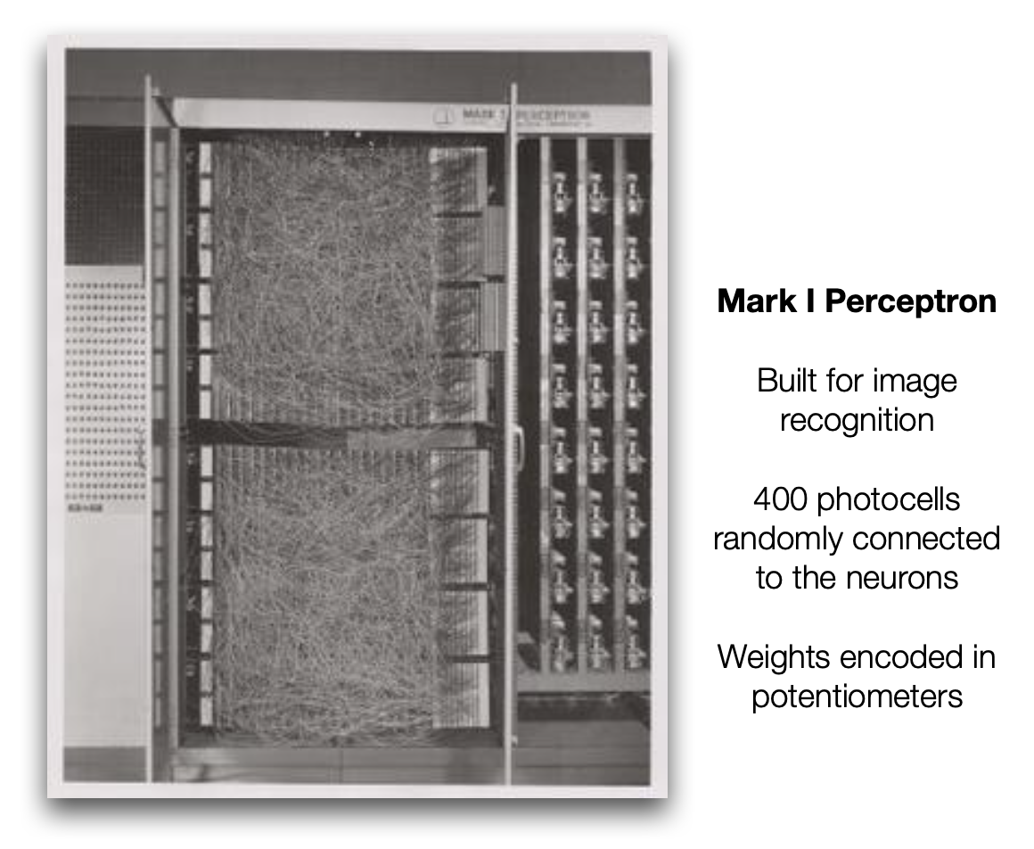
5.13 Rosenblatt’s Perceptron Model
Frank Rosenblatt4 ’s perceptron model was the first one with variable weights that were learned from examples: learning the weights of categories given examples of those categories.
The perceptron was intended to be a machine rather than a program.
First implementation was actually for IBM 704.
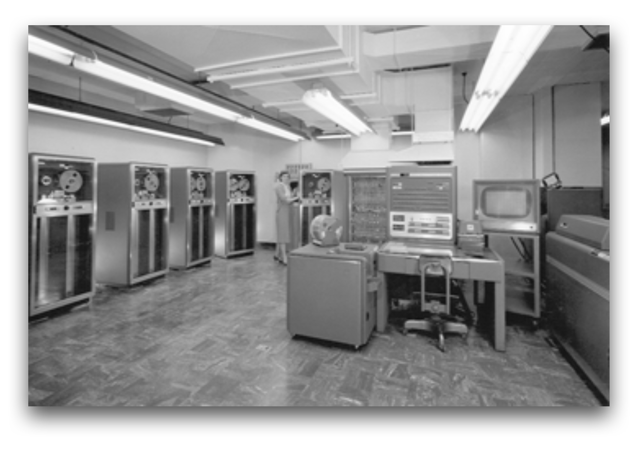
IBM 704
5.14 Limitations of Perceptrons
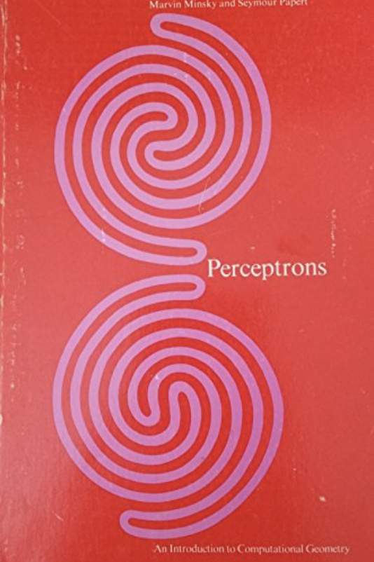
Linear models have many limitations.
Mostly famously, they cannot learn the XOR function where
\(\qquad f([0,1],w) = 1 \quad\) and \(\quad f([1,0],w) = 1\)
but
\(\qquad f([1,1], w) = 0\quad\) and \(\quad f([0,0], w) = 0\)This was observed by Minsky5 and Papert6 in 1969 in Perceptrons.
This was the first major dip in the popularity of neural networks.
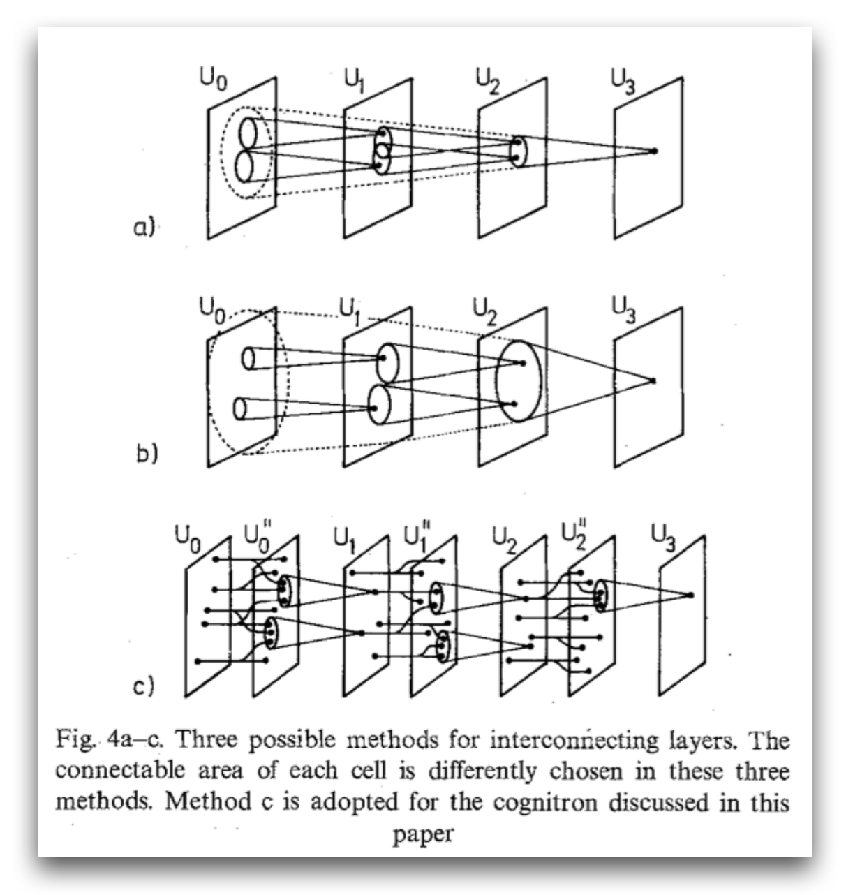
5.15 Neurocognitron and Convolutional Neural Networks
Neuroscience can be an inspiration for the design of novel architectures and solutions.
The basic idea of having multiple computational units that become intelligent via their interactions with each others is inspired by the brain.
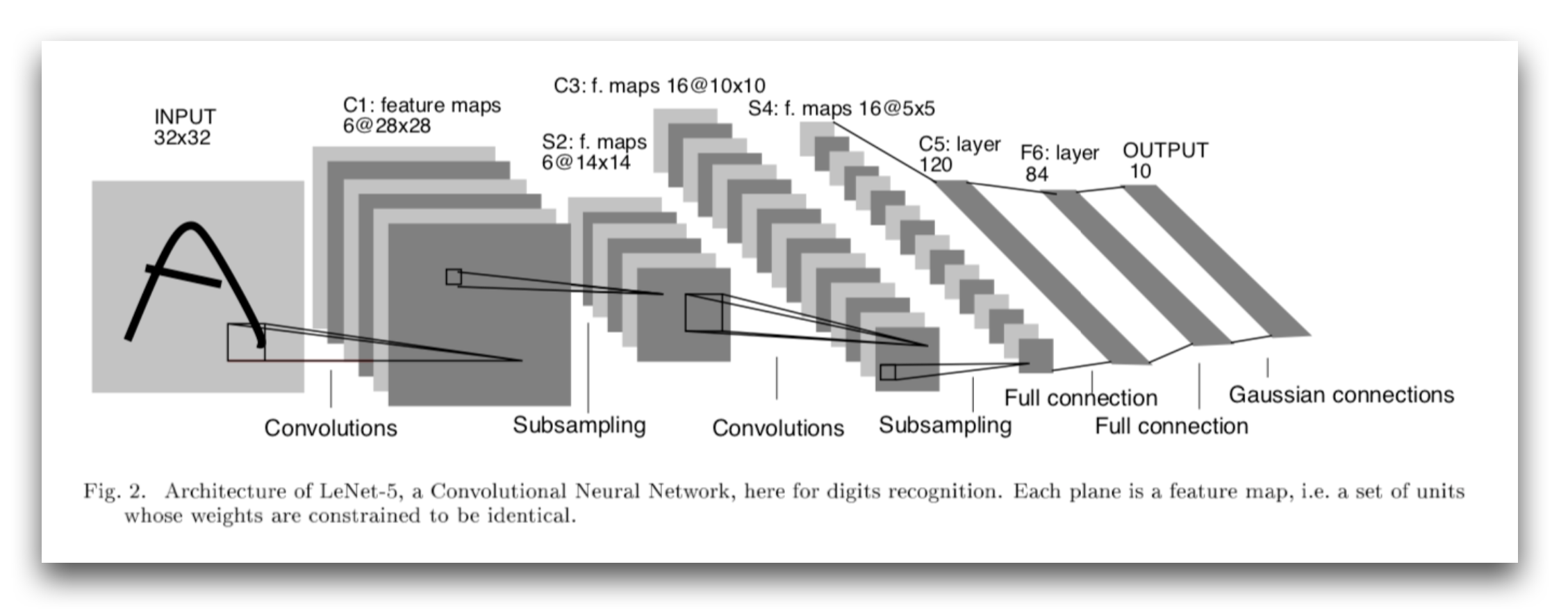
The neurocognitron introduced by Fukushima can be considered as a basis for the modern convolutional networks architectures.
The neurocognitron was the basis of the modern convolutional network architectures (see Yann LeCun et al.’s LeNet architecture).
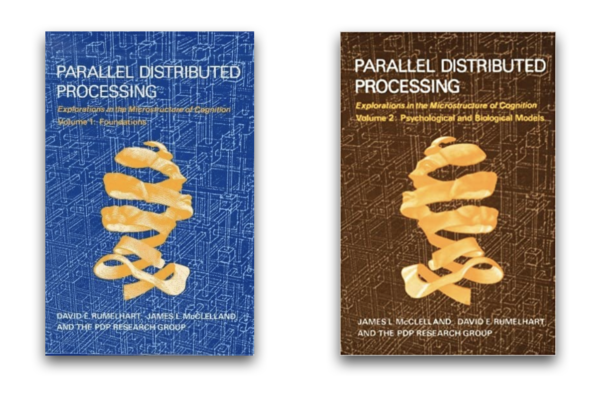
5.16 Connectionism
The second wave of neural network research was in 1980s and started in the cognitive science. It was called connectionism or parallel distributed processing.
- This followed the first winter (mid 70s – 1980).
The focus was on devising models of cognition combining symbolic reasoning and artificial neural network models.
Many ideas are inspired by Hebb’s models.
The idea of distributed representation, i.e., using the raw data without devising features or pre-categorisation of the inputs was introduced by this research movement.
The other key contribution of connectionism was the development of the back- propagation algorithm for training neural networks, which is central in deep learning.
5.17 Second AI Winter and Current AI Summer
The second wave of neural networks lasted until mid 1990s.
- Loss of interest and lot of disappointment due to unrealistic goals led to a new “winter”.
During the second winter, a lot of work continued especially in Canada (and NYU).
The summer returned in 2006 when Geoffrey Hinton7 showed that a particular neural network called a deep belief network could be very efficiently trained (the strategy is called greedy layer-wise pre-training).
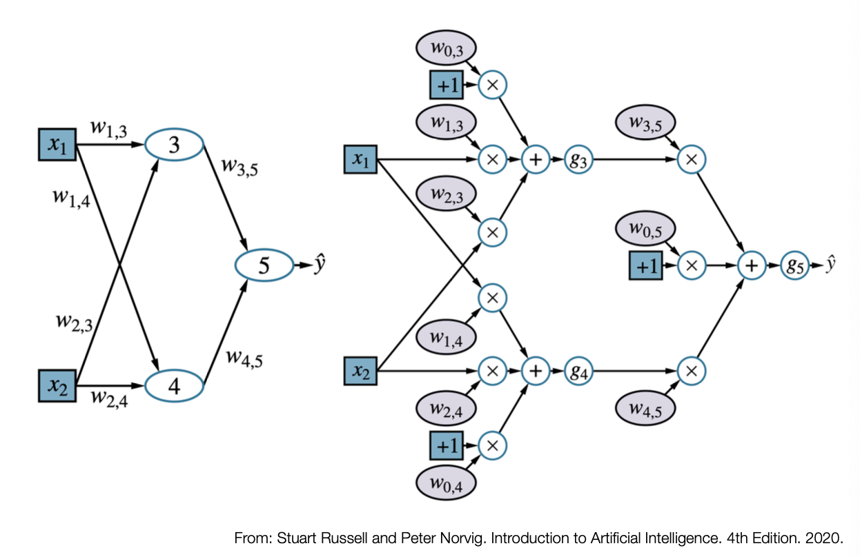
5.18 Networks and Computational Graphs
5.19 Deep Learning Applications
The number of application of deep learning is increasing everyday:
- Image and video processing and vision;
- Machine translation;
- Speech generation;
- Applications to many scientific fields (astronomy, biology, etc.).
- See for example the problem of protein folding.
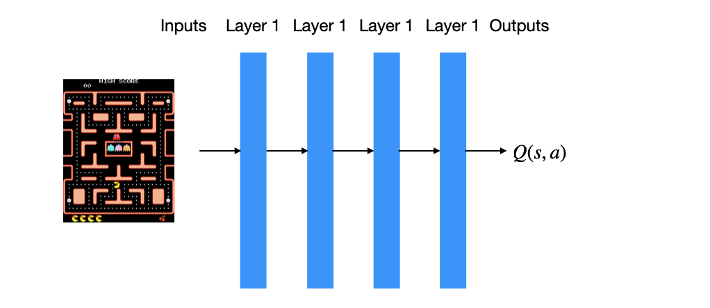
One of the biggest achievement is the extension of the domain of reinforcement learning.
- We refer to the convergence of deep learning and reinforcement learning as deep reinforcement learning.
- Applications of deep reinforcement learning include games, robotics, etc.
5.20 Convolutional Networks
Convolutional networks are networks that contain a mix of convolutional layers, pooling layers and dense layers.
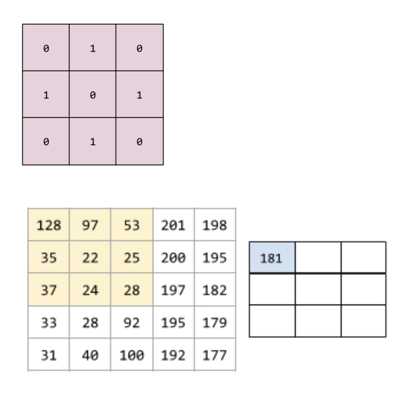
A convolutional layer is a layer of deep neural network, which contains a convolutional filter.
A convolutional filter is a matrix having the same rank as the input matrix but a smaller shape.
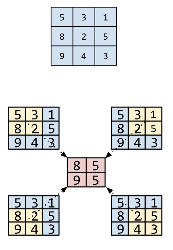
A pooling layer reduces a matrix (or matrices) created by an earlier convolutional layer to a smaller matrix. Pooling usually involves taking either maximum or average value across the pooled area.
A pooling operation divides the matrix into slices and then slides that convolutional operation by strides.
A stride is the delta in each dimension of the convolutional operation.
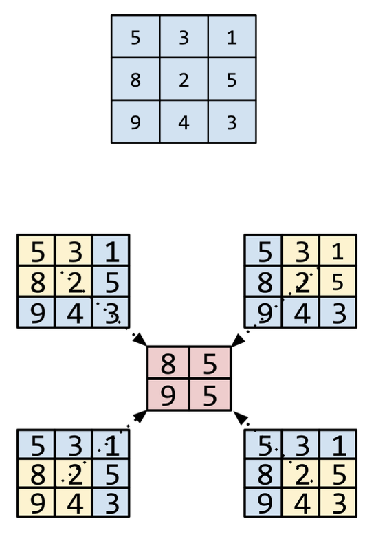
Pooling helps enforce translational invariance, which allows algorithms to classify images when the position of the objects within the images change, in the input matrix.
Pooling for vision applications is usually called spatial pooling.
Pooling for time-series applications is usually referred to as temporal pooling.
We can also hear the expressions subsampling and downsampling.
5.21 Recurrent Neural Networks
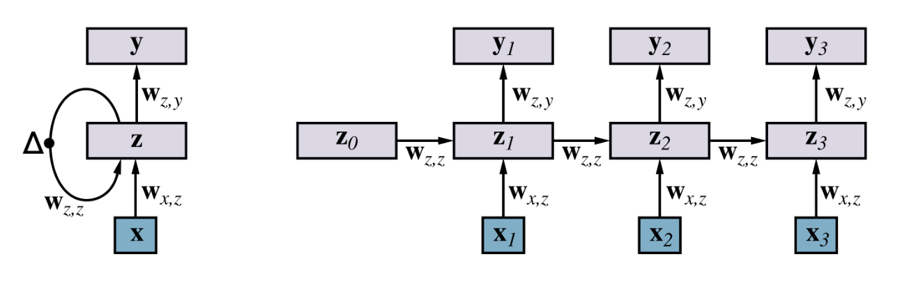
LSTMs
The LSTM is a kind of RNN that down not suffer from the problem of vanishing gradients.
It stands for long short-term memory: it is a kind of RNN with gating units.
In fact, an LSTM can choose to remember part of the input copying it over to the next time step and to forget other parts.
5.22 Residual Networks
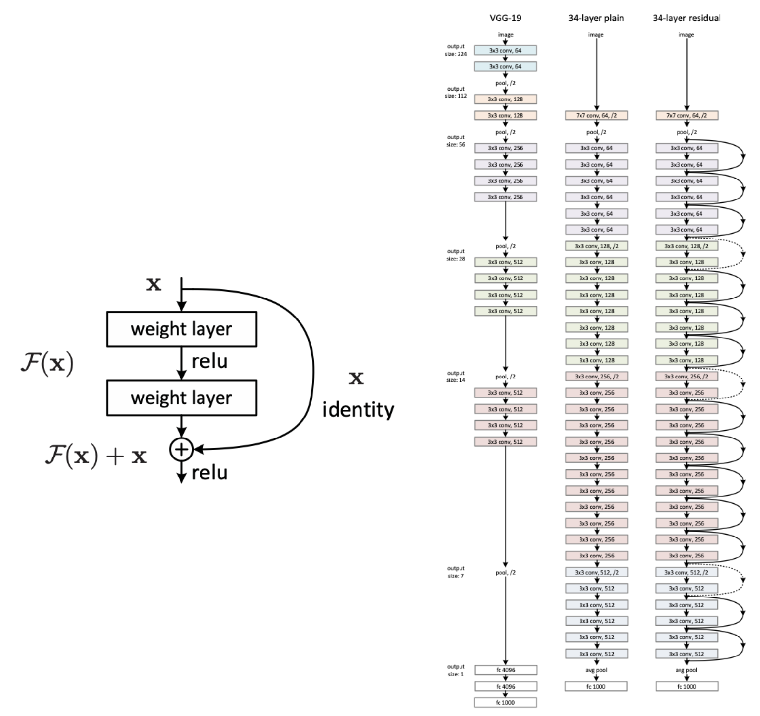
5.23 Neuroscience and Deep Learning
Some Caveats
Neuroscience can be an inspiration, but we should remember that we are trying to “engineer” a system.
Actual neurons are not based on the simple functions that we use in our systems.
- At the moment, more complex functions haven’t led to improve performance yet.
Neuroscience has inspired the design of several neural architectures, but our knowledge is limited in terms of how the brain actually learn.
- For this reason, neurosciece is of limited help for improving the design of the learning algorithms themselves.
Deep learning is not an attempt to simulate the brain!
Deep Learning and Computational Neuroscience
At the same time, it is worth noting that there is an entire field of neuroscience devoted to understanding the brain using mathematical and computational models. The area is called computational neuroscience.
AI and neuroscience are strictly linked and indeed understanding brain biology will lead to improvement in the design of AI systems.
This is currently an area of intense research.
5.24 Superintelligence
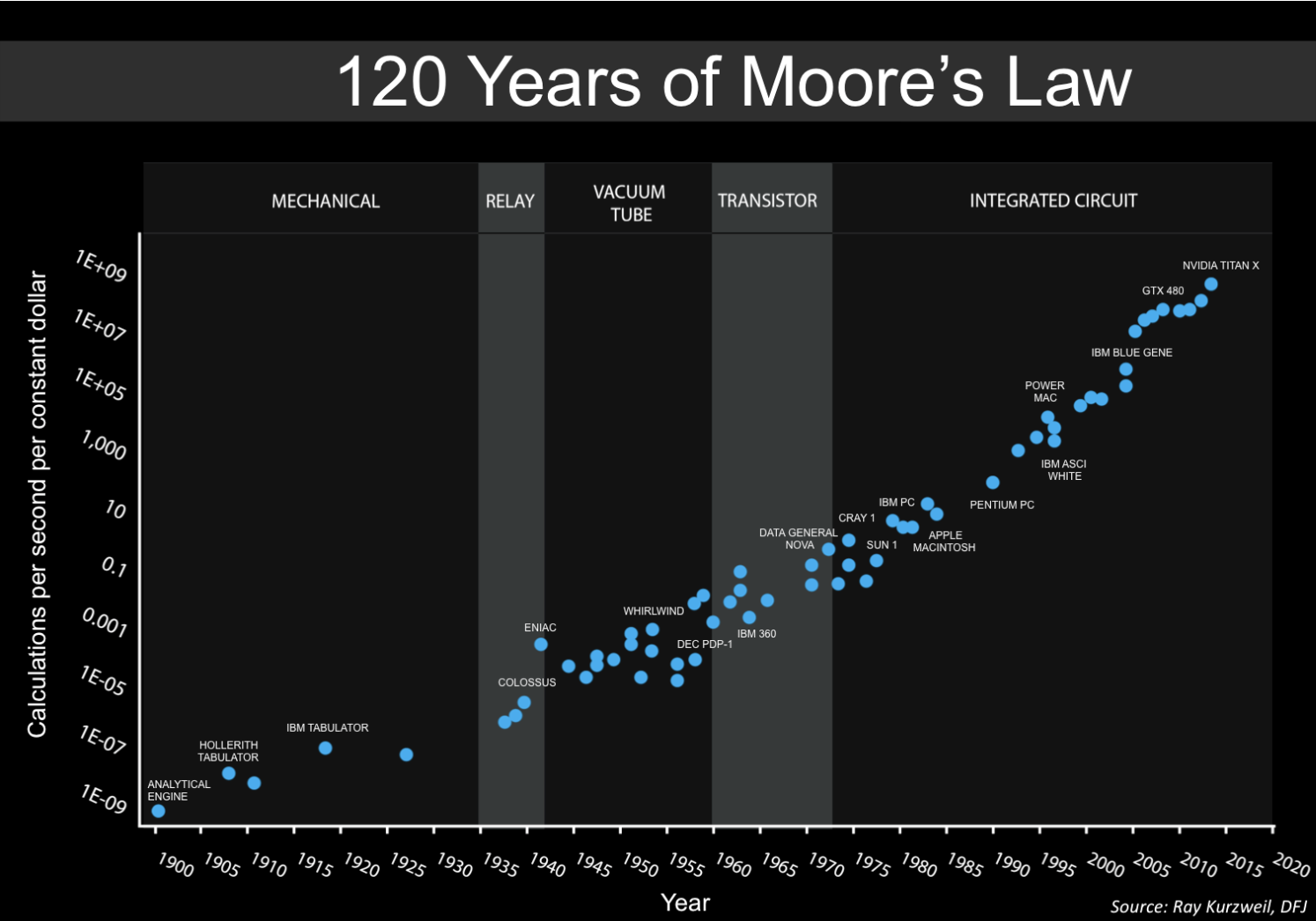
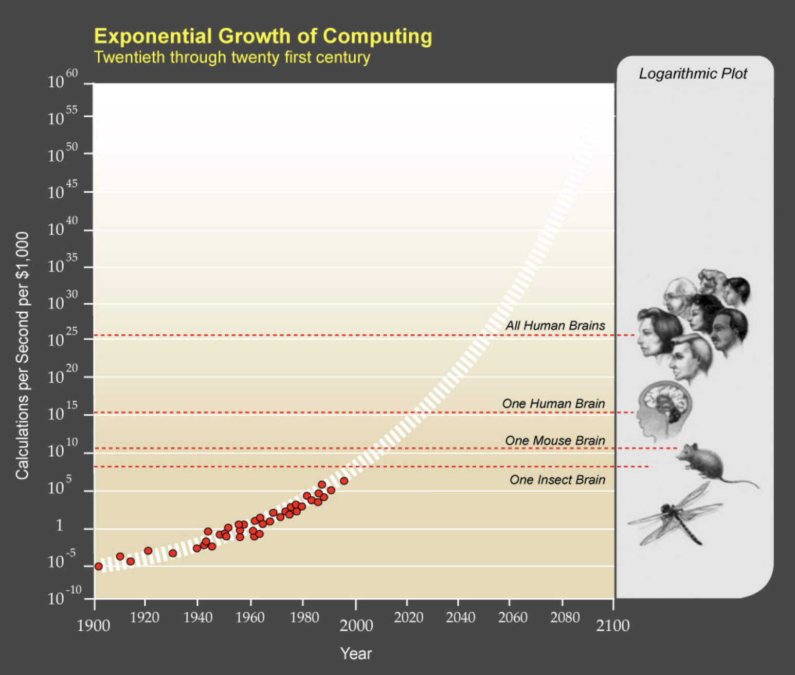
5.25 Is the Singularity near?
5.26 Conscious Machines
5.27 Alternative Minds
5.28 The Brain-Computer Metaphor
5.29 Deep Neural Networks
5.30 Nodes/Units/Neurons
5.31 Activation Functions
Activation functions are generally used to add non-linearity.
Examples:
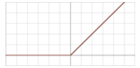
- Rectified Linear Unit (\(relu\)): it returns the max between \(0\) and the value in input. In other words, given the value \(z\) in input it returns \(max(0,z)\).
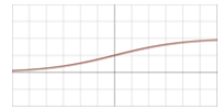
- Logistic sigmoid: given the value in input \(z\)m it returns \(\frac{1}{1 + e^z}\).
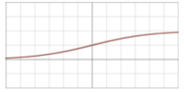
- Arctan: given the value in input \(z\), it returns \(\tan^{-1}(z)\).
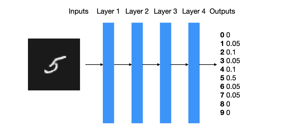
5.32 Softmax Function
Another relevant function is softmax.
It is not like the activation functions discussed before, as they take in input real numbers and return a real number.
A softmax function receives in input a vector of real numbers of dimensin \(n\) and returns a vector of real numbers of dimension \(n\).
Softmax: given a vector of real numbers in input \(\mathrm{z}\) of dimension \(n\), it normalises it into a probability distribution consisting of \(n\) probabilities proportional to the exponentials fo each element \(z_i\) of the vector \(\mathrm{z}\). More formally:
\(softmax(\mathrm{z})_i = \frac{e^{z_i}}{\sum^n_{j=1}e^{z_i}}\) for \(i = 1, \dots, n\).
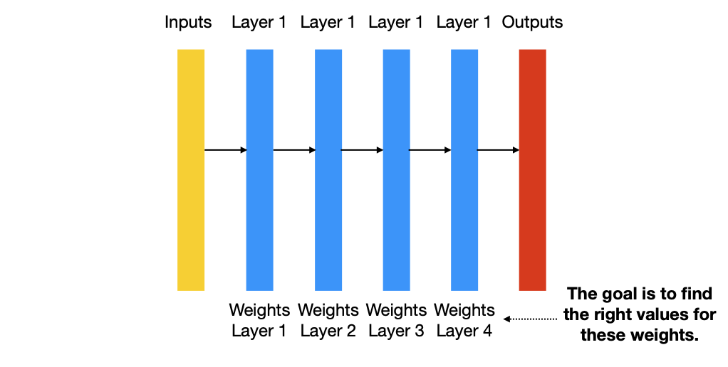
5.33 Gradient-based Optimisation
We will now discuss a high-level description of the learning process of the network, usually called gradient-based optimization.
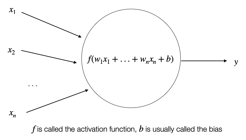
Each neural layer transforms his input layer as follows:
\(output = f(w_1 x_1 + \dots + w_n x_n + b)\)
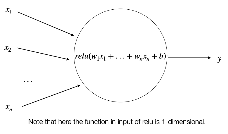
And in the case of a relu function, we will have
\(output = relu(w_1 x_1 + \dots + w_n x_n + b)\)
Notice that this is a simplified notation for one layer, it should be \(w_{1,i}\) for layer \(i\).
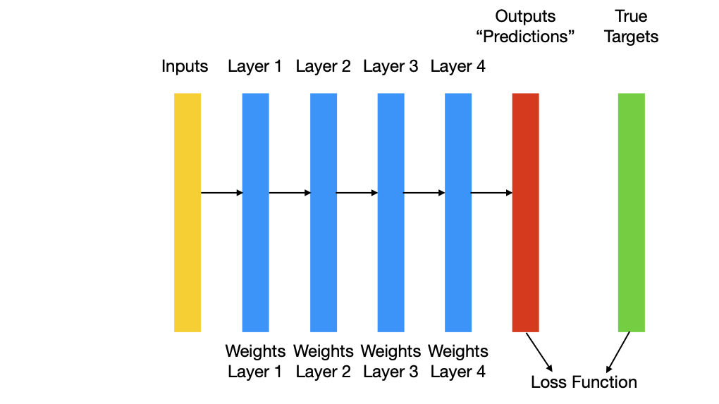
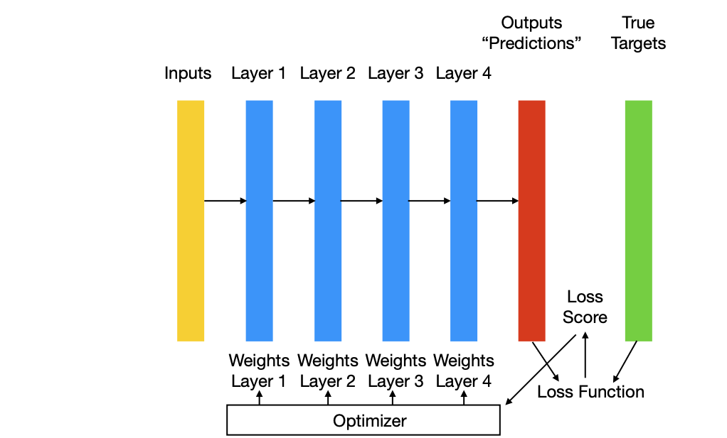
The learning is based on the gradual sdjustment of the weight based on a feedback signla, i.e. the loss described above.
The training is based on the following training loop:
Draw a batch of training examples \(\mathrm{x}\) and corresponding targets \(\mathrm{y}_{target}\).
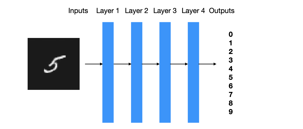
Run the network on \(\mathrm{x}\) (forward pass) to obtain predictions \(\mathrm{y}_{pred}\).
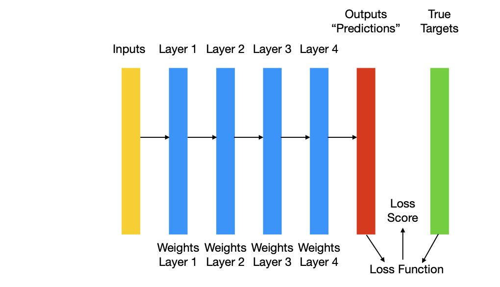
Compute the loss of the network on the batch, a measure of the mismatch between \(\mathrm{y}_{pred}\) and \(\mathrm{y}_{target}\).
Update all weights of the networks in a way that reduces the loss of this batch.
Stochastic Gradient Descent
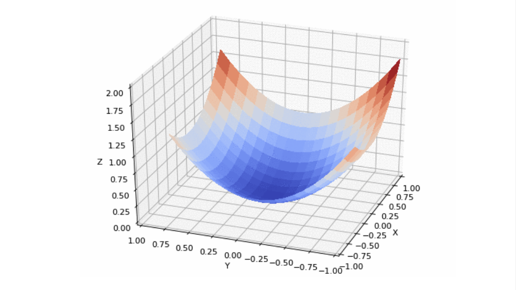
Given a differentiable function, it’s theoretically possible to find its minimum analytically.
However, the function is interactable for real networks. The only way is to try to approximate the weights using the procedure described above.
More precisely, since it is a differentiable function, we can use the gradient, which provides an efficient way to perform the correction mentioned before.
More formally:
Draw a batch of training examples \(\mathrm{x}\) and corresponding targets \(\mathrm{y}_{target}\).
Run the network on \(\mathrm{x}\) (forward pass) to obtain predictions \(\mathrm{y}_{pred}\).
Compute the loss of the network on the batch, a measure of the mismatch between \(\mathrm{y}_{pred}\) and \(\mathrm{y}_{target}\).
Compute the gradient of the loss with regard to the network’s parameters (backward pass).
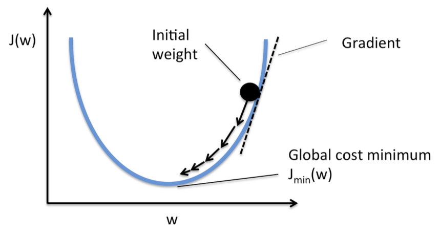
Move the parameters in the opposite direction from the gradient with:
\[w_j \leftarrow w_j + \nabla w_j = w_j - \mu \frac{\delta J}{\delta w_j}\] \(\qquad\) where \(J\) is the loss (cost) function.
- If we have a batch of samples of dimension \(k\):
\[w_j \leftarrow w_j + \nabla w_j = w_j - \mu \; average(\frac{\delta J_k}{\delta w_j})\] \(\qquad\) for all the \(k\) samples of the batch.
This is called the mini-batch stochastic gradient descent (mini-batch SGD).
The loss function \(J\) is a function of \(f(\mathrm{x})\), which is a function of the weights.
Essentially, we calculate the value \(f(\mathrm{x})\), which is a function of the weights of the network.
Therefore, by definition, the derivative of the loss function that we are going to apply will be a function of the weights.
The term stochastic refers to the fact that each batch of data is drawn randomly.
The algorithm described above was based on a simplified model with a single function in a sense.
We can think about a network composed of three layers, e.g. three tensor operations on the network itself.
5.34 Backpropagation Algorithm
Suppose that we have three tensor operations/layers \(f,g,h\) with weights \(\mathrm{W}^1, \mathrm{W}^2\) and \(\mathrm{W}^3\) respectivaly for the first, second, third layer. We will have the following function:
\[y_{pred} = f(\mathrm{W}^1, \mathrm{W}^2, \mathrm{W}^3, \mathrm{x}) = f(\mathrm{W}^3, g(\mathrm{W}^2, h(\mathrm{W}^1, \mathrm{x})))\]
with \(f()\) the rightmost fucntion/layer and so on.
In other words, the input layer is connected to \(h()\), which is connected to \(g()\), which is connected to \(f()\), which returns the final result.
A network is a sort of chain of layers. We can derive the value of the “correction” by applying the chain rule of the derivatives backwards.
Remember the chain rule:
\((f(g(x)))' = f'(g(x))\;g'(x)\)
The update of the weights starts from the right-most layer back to the left-most layer. For this reason, this is called backpropagation algorithm.
More specifically, backpropagation starts with the calculation of the gradient of final loss value and works backwards from the right-most layers to the left-most layers, applying the chain rule to compute the contribution that each weight had in the loss value.
Nowadays, we do not calculate the partial derivatives manually, but we use frameworks like TensorFlow and PyTorch that support symbolic differentiation for the calculation of the gradient.
TensorFlow and PyTorch support the automatic updates of the weights described above.
\(\blacktriangleright\) More theoretical details can be found in Goodfellow, Bengio, and Courville (2016).
5.35 Attribution Notice
Portion of the material in this section about convolutional networks, recurrent networks are modifications based on work created and shared by Google and used according to terms described in the Creative Commons 4.0 Attribution License.
\(\blacktriangleright\) Source: developers.google.com/machine-learning/glossary/
\(\blacktriangleright\) Attribution license: creativecommons.org/licenses/by/4.0/
5.36 References
5.37 Pointers about Neural Network Calibration
Chuan Guo, Geoff Pleiss, Yu Sun, Kilian Q. Weinberger. On Calibration of Modern Neural Networks. Proceedings of the 34th International Conference on Machine Learning (ICML 2017).
\(\blacktriangleright\) Amazon AWS article on temperature scaling
\(\blacktriangleright\) TensorFlow class for Expected Calibration Error (see paper above for definitions, etc)
Warren McChulloch (1898 – 1969): https://it.wikipedia.org/wiki/Warren_McCulloch↩︎
Walter Pitts (1923 – 1969): https://it.wikipedia.org/wiki/Walter_Pitts↩︎
Donald Olding Hebb (1904 – 1985): https://it.wikipedia.org/wiki/Donald_Olding_Hebb↩︎
Frank Rosenblatt (1928 – 1971): https://it.wikipedia.org/wiki/Frank_Rosenblatt↩︎
Marvin Minsky (1927 – 2016): https://it.wikipedia.org/wiki/Marvin_Minsky↩︎
Seymour Papert (1928 – 2016): https://it.wikipedia.org/wiki/Seymour_Papert↩︎
Geoffrey Everest Hinton (1947): https://it.wikipedia.org/wiki/Geoffrey_Hinton↩︎